covid <- read_covid() %>%
  arrange(date) %>%
  mutate(daily_cases = confirmed - lag(confirmed, default = 0))

covid %>%
  select(date, confirmed, daily_cases) %>%
  slice(85:90)
#> # A tibble: 6 × 3
#>   date       confirmed daily_cases
#>   <date>         <dbl>       <dbl>
#> 1 2020-04-15      3699         447
#> 2 2020-04-16      4427         728
#> 3 2020-04-17      5050         623
#> 4 2020-04-18      5992         942
#> 5 2020-04-19      6588         596
#> 6 2020-04-20 8014 14267 Making decisions
Much of routine epidemiological reporting turns numbers into labels: a count of 1,426 becomes a high day before it reaches a bulletin. R provides two different tools for this. One decides what the script does next; the other decides what goes in a column. Using the first where the second is needed produces either an error or, less visibly, a result that is correct for one row and wrong for the other 344.
This chapter distinguishes the two, then uses the second to build a severity label for every day of 2020.
7.1 Where we are
Everything here starts from the daily counts you built in the previous chapter. The file ships cumulative totals, so a day’s new cases is today’s total minus yesterday’s, and lag(confirmed, default = 0) supplies the “yesterday” for the very first row. That default matters: confirmed is 0 on 22 January, so day one had a real zero of new cases, not a missing one.
7.2 if tests a single value
R’s if is a control-flow statement. It looks at a single TRUE or FALSE and picks which block of code to run. It is the appropriate tool when the decision is about the analysis as a whole.
worst <- max(covid$daily_cases)
worst
#> [1] 1426

if (worst > 1000) {
  "Singapore recorded a four-figure day."
} else {
  "No day reached a thousand."
}
#> [1] "Singapore recorded a four-figure day."
worst is one number, so worst > 1000 is a single TRUE and if can act on it.
Suppose instead you want a label on every row, and write the version that reads like English:
if (covid$daily_cases > 300) "High" else "Not high"
#> Error in `if (covid$daily_cases > 300) ...`:
#> ! the condition has length > 1
covid$daily_cases > 300 is not a single TRUE or FALSE but a vector of 345 of them.
length(covid$daily_cases > 300)
#> [1] 345
if has no way to act on 345 answers at once, so it refuses. The message to search for is the condition has length > 1.
Up to R 4.1 the same code ran: R issued a warning, took the first element and carried on. A script could label an entire dataset “Not high” because 22 January happened to have zero cases, with only a warning to indicate it. R 4.2 made this an error, so a script written against the earlier behaviour stops here on any current version of R.
When you do want a whole-dataset question, collapse the vector to one value first. any() and all() are built for this.
if (any(covid$daily_cases > 1000)) {
  "At least one day topped a thousand."
}
#> [1] "At least one day topped a thousand."
7.3 if_else() builds a column
For a label on every row you want a vectorised choice: one input vector in, one output vector out, same length. dplyr’s if_else() does that.
covid %>%
  mutate(big_day = if_else(daily_cases > 300, "High", "Not high")) %>%
  count(big_day)
#> # A tibble: 2 × 2
#>   big_day      n
#>   <chr>    <int>
#> 1 High        77
#> 2 Not high   268
Read the arguments as a sentence: for each row, test daily_cases > 300; where it is TRUE use "High", where it is FALSE use "Not high".
if_else() requires both branches to be of the same type, and the requirement is deliberate:
covid %>%
  mutate(big_day = if_else(daily_cases > 300, "High", 0))
#> Error in `mutate()` at magrittr/R/pipe.R:136:3:
#> ℹ In argument: `big_day = if_else(daily_cases > 300, "High", 0)`.
#> Caused by error in `if_else()`:
#> ! Can't combine `true` <character> and `false` <double>.
Can’t combine true false if_else() does not choose between them. Base R’s ifelse() does choose, by coercing both branches to a common type, and the coercion drops attributes. The effect on a date column:
Those five-digit numbers are days since 1 January 1970, which is how R stores a Date underneath. ifelse() stripped the class attribute and handed back the raw numbers, so a date column comes out as a numeric one.
if_else(big$daily_cases > 300, big$date, as.Date(NA))
#> [1] "2020-04-13" "2020-04-14" "2020-04-15"
if_else() keeps the class of the branches it returns, so the same comparison comes back with the dates intact.
7.4 case_when() when there are more than two answers
Each label beyond the second adds another test, and nesting if_else() inside if_else() produces code that is hard to read and harder to check. case_when() replaces the nesting with a list of conditions, each paired with the value to use when it matches.
The course uses three cutoffs: under 100 new cases is Low, 100 up to and including 300 is Medium, and over 300 is High.
covid <- covid %>%
  mutate(
    # Course convention: fewer than 100 cases is Low, 100 up to and
    # including 300 is Medium, over 300 is High.
    severity = case_when(
      daily_cases <  100 ~ "Low",
      daily_cases <= 300 ~ "Medium",
      daily_cases >  300 ~ "High"
    )
  )

covid %>% count(severity)
#> # A tibble: 3 × 2
#>   severity     n
#>   <chr>    <int>
#> 1 High        77
#> 2 Low        215
#> 3 Medium      53
The ~ separates the test from the result. R uses the tilde wherever the two sides of a relationship have to sit in one expression, which is why it also appears in modelling formulas and in ggplot facet specifications; inside case_when() it means “gives”.
case_when() works top to bottom and first match wins. Once a row matches a line, later lines never see it. That is what lets the second condition be daily_cases <= 300 and not daily_cases >= 100 & daily_cases <= 300: any row still being tested on line two already failed line one, so it already has at least 100 cases.
The order of the lines therefore matters. Swapping the first two leaves the arithmetic identical and the answer different:
covid %>%
  mutate(
    wrong = case_when(
      daily_cases <= 300 ~ "Medium",
      daily_cases <  100 ~ "Low",
      daily_cases >  300 ~ "High"
    )
  ) %>%
  count(wrong)
#> # A tibble: 2 × 2
#>   wrong      n
#>   <chr>  <int>
#> 1 High      77
#> 2 Medium   268
Because the Medium line is evaluated first, it matches every Low day as well, and 215 days are mislabelled with no error and no warning. When a case_when() returns a category with a count of zero, or one much larger than expected, the order of the conditions is the first thing to check.
The other failure mode is a row that matches nothing at all. Drop the last line and the 77 High days match no condition:
covid %>%
  mutate(
    incomplete = case_when(
      daily_cases <  100 ~ "Low",
      daily_cases <= 300 ~ "Medium"
    )
  ) %>%
  count(incomplete)
#> # A tibble: 3 × 2
#>   incomplete     n
#>   <chr>      <int>
#> 1 Low          215
#> 2 Medium        53
#> 3 <NA>          77
case_when() returns NA for unmatched rows rather than complaining, so this only shows up if you look. .default catches everything that falls through; use it whenever your conditions are meant to be exhaustive:
covid %>%
  mutate(
    severity_alt = case_when(
      daily_cases <  100 ~ "Low",
      daily_cases <= 300 ~ "Medium",
      .default = "High"
    )
  ) %>%
  count(severity_alt)
#> # A tibble: 3 × 2
#>   severity_alt     n
#>   <chr>        <int>
#> 1 High            77
#> 2 Low            215
#> 3 Medium          53
Two details of that block deserve to stick. The recoded column gets a new name, severity_alt, rather than overwriting severity, so both versions remain available to count side by side while you check the change. The category labels are also spelled exactly as the existing column has them, because later steps match text literally: a lower-case "high" would start a fourth category rather than match "High".
7.5 Boundary values
“100 to 300” is ambiguous in English and unambiguous in code, so writing the code forces a decision that the specification may have left open: a day with exactly 100 cases could be Low or Medium, and 300 could be Medium or High. The case_when() settles both questions one way or the other, so choose the convention deliberately.
This dataset contains days sitting on both ends of the rule.
Predict before you run
Consider two days in August: 18 August had exactly 100 new cases, and 6 August had 301. Under the cutoffs written above, write down the label each of them gets before you look. Check the boundary cases: they are where an off-by-one in the cutoffs shows up.
18 August is Medium because daily_cases < 100 is FALSE at exactly 100, so the day falls through to the <= 300 line; 6 August is High because 301 is one case past <= 300. Changing < to <= on the first line moves 18 August to Low, so a single character changes the label on a day that occurs in the data.
Write the thresholds down in prose next to the code, with the inequalities spelled out, as the comment in the case_when() block above does. “Fewer than 100” and “up to 100” are different rules, and they disagree on days that occur in this dataset.
7.6 Missing values fall straight through
Neither if_else() nor case_when() treats NA as FALSE. NA > 0 is NA, which is neither branch, so the result is NA. Deaths in this file are missing for the first 59 days, so they show it plainly:
covid %>%
  mutate(
    daily_deaths = deaths - lag(deaths, default = 0),
    death_day = if_else(daily_deaths > 0, "yes", "no")
  ) %>%
  count(death_day)
#> # A tibble: 3 × 2
#>   death_day     n
#>   <chr>     <int>
#> 1 no          260
#> 2 yes          25
#> 3 <NA>         60
Sixty rows came back NA: the 59 days before any death total was published, plus the first day that had one, which has no valid predecessor to difference against. if_else() gives you a missing = argument to label them explicitly:
covid %>%
  mutate(
    daily_deaths = deaths - lag(deaths, default = 0),
    death_day = if_else(daily_deaths > 0, "yes", "no", missing = "not reported yet")
  ) %>%
  count(death_day)
#> # A tibble: 3 × 2
#>   death_day            n
#>   <chr>            <int>
#> 1 no                 260
#> 2 not reported yet    60
#> 3 yes                 25
In case_when() you do the same thing with an is.na() line placed first, so that missing rows are matched before any comparison has a chance to return NA. This keeps “no deaths reported” distinct from “deaths not yet reported”; the two are different findings, and a table that merges them into one category misleads.
7.7 Ordering categories with factor()
count() is the dplyr way of tabulating a column. Base R’s table() does the same job in less typing, and it returns a named vector of counts instead of a data frame. Look at the order it puts the labels in:
table(covid$severity)
#>
#>   High    Low Medium
#>     77    215     53
The counts come back in alphabetical order — High, Low, Medium — which for an ordered variable carries no meaning. Alphabetical order puts the most severe category first and the middle category last, and any bar chart, legend or summary table built from that column inherits the same ordering.
R sorts alphabetically because severity is currently plain text:
class(covid$severity)
#> [1] "character"
A character vector has no order other than the alphabetical one. factor() records that these three strings are the levels of a categorical variable and fixes the order they are held in.
The counts are 215 Low, 53 Medium and 77 High, and they sum to 345, which is every day of the dataset, so nothing fell through the conditions.
A factor stores small integers plus a lookup table of labels, which is why the ordering sticks:
levels(covid$severity)
#> [1] "Low"    "Medium" "High"
as.integer(head(covid$severity, 5))
#> [1] 1 1 1 1 1
head(covid$severity, 5)
#> [1] Low Low Low Low Low
#> Levels: Low Medium High
Rows 1 to 5 are stored as 1, displayed as Low, and sorted first because Low is level one. ggplot reads exactly the same information, so the same fix that repairs table() repairs your axes:
p_chr <- ggplot(covid, aes(x = as.character(severity))) +
  geom_bar() +
  labs(title = "Stored as text", x = NULL, y = "Days")

p_fct <- ggplot(covid, aes(x = severity)) +
  geom_bar() +
  labs(title = "Stored as a factor", x = NULL, y = "Days")

p_chr + p_fct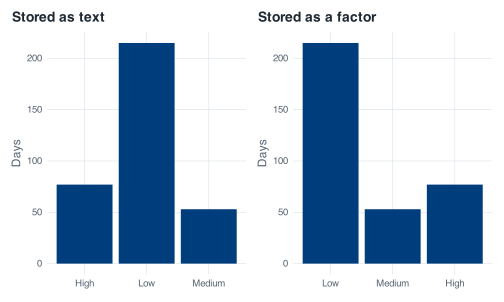
The same problem arises for age bands, Likert scales, disease stages, income quintiles, and WHO regions ordered by anything other than the alphabet. Each of them arrives as text, and each needs factor(levels = ...) before it tabulates or plots in the intended order.
There is one caution: factor() converts any value not listed in levels to NA, without a warning, including a value that differs only in case:
head(factor(as.character(covid$severity), levels = c("low", "Medium", "High")))
#> [1] <NA> <NA> <NA> <NA> <NA> <NA>
#> Levels: low Medium High
table(factor(as.character(covid$severity), levels = c("low", "Medium", "High")), useNA = "ifany")
#>
#>    low Medium   High   <NA>
#>      0     53     77    215
Because the levels say "low" where the data has "Low", all 215 Low days become NA, without a warning. After creating a factor, run table(..., useNA = "ifany") or count() once and check that the total still matches the number of rows.
7.8 The dataset, assembled
Putting the pieces together, here is the whole thing in one block: the file as it ships, sorted by date, with daily counts differenced out of the cumulative columns, a severity factor in sensible order, and a month column produced by rounding each date down to the first of its month.
covid <- read_covid() %>%
  arrange(date) %>%
  mutate(
    daily_cases  = confirmed - lag(confirmed, default = 0),
    daily_deaths = deaths - lag(deaths, default = 0),
    severity = case_when(
      daily_cases <  100 ~ "Low",
      daily_cases <= 300 ~ "Medium",
      daily_cases >  300 ~ "High"
    ),
    severity = factor(severity, levels = c("Low", "Medium", "High")),
    month = floor_date(date, "month")
  )

covid %>%
  select(date, daily_cases, daily_deaths, severity, month) %>%
  slice(85:88)
#> # A tibble: 4 × 5
#>   date       daily_cases daily_deaths severity month
#>   <date>           <dbl>        <dbl> <fct>    <date>
#> 1 2020-04-15         447            0 High     2020-04-01
#> 2 2020-04-16         728            0 High     2020-04-01
#> 3 2020-04-17         623            1 High     2020-04-01
#> 4 2020-04-18         942            0 High     2020-04-01
That block is what covid_daily() runs. Its definition sits in _common.R in the project root, where you can open and read it, so covid <- covid_daily() rebuilds this table in one line in a fresh session. It contains nothing beyond what you have now built by hand.
7.9 Exercises
Exercise 7.1 (Audit your severity column) Check the severity column before relying on it.
- Confirm the three counts add up to 345 and that no day came back
NA. - For each label, report the smallest and the largest
daily_casesit contains. - Look at the numbers from step 2 either side of each cutoff, and say how far you could move the 100 threshold, in either direction, before a single day changed its label.
For step 3, write down what the answer tells you about how far the labelling depends on the exact value 100.
Stuck? Open for a hint (not the answer)
group_by(severity) followed by a summarise() containing n(), min() and max() answers steps 1 and 2 in one call: group_by() splits the rows into one pile per label, and summarise() computes one row of answers for each pile. If you would rather stay with verbs you have already used, a filter() per label and a range() on each gets you the same three pairs of numbers with more typing. For the NA check, count() shows a missing category if one exists.
Exercise 7.2 (Move the cutoffs) The 100 and 300 thresholds are a convention adopted for this course, and other cutoffs are equally defensible. Rebuild severity with cutoffs at 50 and 500 instead, keeping the same boundary conventions (under 50 is Low, 50 up to and including 500 is Medium, over 500 is High).
Report the three counts under the new rule, and compare them with 215 / 53 / 77. Then write two sentences you would be willing to put in a report under each set of cutoffs, describing how severe 2020 was. Both sentences must be true of the same 345 days.
Stuck? Open for a hint (not the answer)
Copy the case_when() block, change the two numbers, and give the new column a different name so you can count() both and put the results side by side. Do not forget the factor() line, or your new column will sort alphabetically again.