ggplot(covid, aes(x = date, y = confirmed)) +
  geom_line()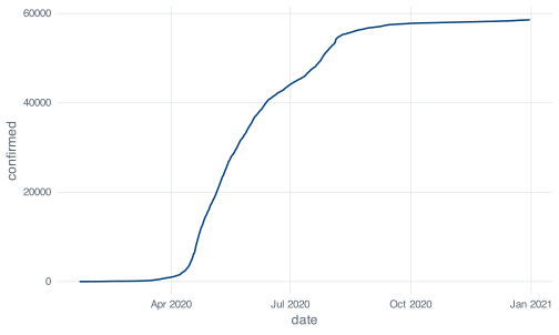
A plot is the quickest visible result a beginner gets from R, which is why plotting is often taught first. This chapter comes later, after you have learned to reshape a data frame, for a reason specific to the file on your disk: none of its thirteen columns holds the daily case counts you would put on the y axis of an epidemic curve. confirmed is a running total, and a running total of an epidemic looks like this:
ggplot(covid, aes(x = date, y = confirmed)) +
geom_line()That curve is accurate, and there is very little to read off it. Cumulative curves have much the same shape in every epidemic: flat, then steep, then flat again at a higher level. The circuit breaker is not visible in it, nor is the August reporting artifact, and telling a month with 200 cases apart from a month with 20,000 means reading two values off the axis and subtracting them.
The variable to plot, daily_cases, exists because you built it in an earlier chapter with mutate() and lag(). Teaching ggplot2 before that would have meant demonstrating it on the cumulative column.
ggplot(covid, aes(x = date, y = daily_cases)) +
  geom_line()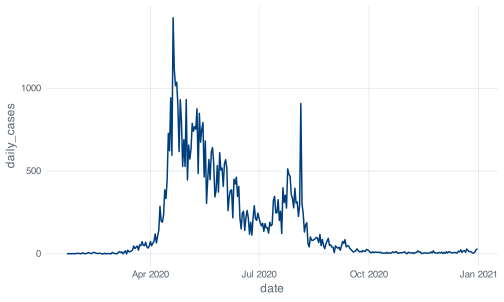
This shows the dormitory outbreak, the effect of the circuit breaker from late April, the long decline through the second half of the year, and the single vertical spike on 5 August. The two figures are drawn from the same file and differ only by the mutate() from the earlier chapter.
Every ggplot2 plot needs three answers before it can draw anything, and the two-line call above supplied all three.
The first is which data frame, and that is the first argument to ggplot(). Every column you name later has to live in it.
The second is which columns go on which visual channel. A channel here means a property the reader can perceive: horizontal position, vertical position, colour, size, shape, transparency. ggplot2 calls these aesthetics, a term that covers position as well as appearance, and you declare the mapping inside aes().
The third is what marks to actually draw: lines, points, bars, or boxes. ggplot2 calls these geoms, and each one is a function whose name starts geom_.
The same call, with each of the three parts labelled:
ggplot(
data = covid,
mapping = aes(x = date, y = daily_cases)
) +
geom_line()date drives horizontal position, daily_cases drives vertical position.
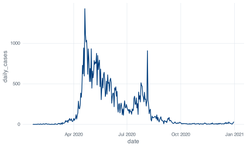
The names data = and mapping = are conventionally omitted, because they are the first two arguments and aes() is unmistakable. ggplot(covid, aes(date, daily_cases)) is the same call. Write the names out while you are learning and drop them when they stop helping you.
Run ggplot(covid, aes(x = date, y = daily_cases)) on its own, with no geom, and you get an empty grey panel with correctly labelled axes. The axes show that the data and the mapping were understood; the empty panel shows that no layer was supplied. Running the call without its geoms is a useful step when a plot comes out wrong, because it separates a broken mapping from a broken geom.
Out of the box, geom_line() draws in black. The line above is NUS blue because _common.R, the setup file every chapter sources, calls update_geom_defaults() to change the default and theme_set(theme_nus()) to change the grid, the fonts and the legend position. That code lives in R/nus_theme.R if you want to read it.
This matters for one practical reason. When you copy a chunk out of this book into your own script and it comes out looking different, the difference is the house theme, not a mistake on your part. The named colours this chapter uses, nus_colours[["crimson"]] and friends, come from the same file and will not exist in a fresh R session.
Inside aes(), you name a column and ggplot2 works out the colours. Outside aes(), you name a colour and ggplot2 uses it. Putting a colour name inside aes() draws without complaint and produces no error message:
ggplot(covid, aes(x = date, y = daily_cases)) +
  geom_line(aes(colour = "red"))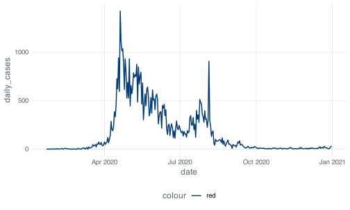
aes(colour = "red") maps the colour channel to a variable whose value is the string red on every row, and ggplot2 treats it as such. It finds one distinct value, assigns it the first colour in the palette, and builds a legend to explain the assignment. The legend title is colour because the mapped expression has no other name.
The version that does what you meant puts the colour outside aes():
ggplot(covid, aes(x = date, y = daily_cases)) +
  geom_line(colour = "red")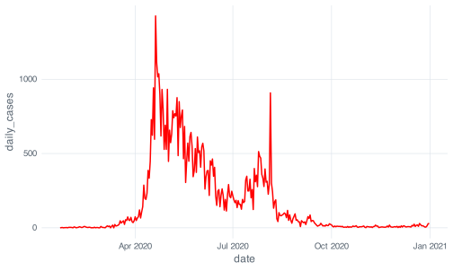
The rule: if the value should change from row to row, it goes inside aes(). If it is one fixed value, it goes outside. An unexpected legend is usually this mistake.
+ adds a layer to a plot. %>% passes an object to a function as its first argument. They are not interchangeable, and swapping one for the other stops the plot from being drawn at all.
ggplot(covid, aes(x = date, y = daily_cases)) %>%
  geom_line()
#> Error in `geom_line()` at magrittr/R/pipe.R:136:3:
#> ! `mapping` must be created by `aes()`.
#> ✖ You've supplied a <ggplot2::ggplot> object.
#> ℹ Did you use `%>%` or `|>` instead of `+`?
Read the error to the end. The first line names the function that failed. The second states the rule that was broken. The third says what was actually supplied. The fourth identifies the likely mistake and names the fix.
Read every line of an R error before returning to your script. Recent tidyverse errors are written to be this specific about the fix. Errors elsewhere in R are often much less informative, and reading the message is how you find out which kind you have.
The historical reason for the split: ggplot2 reached CRAN in 2007, and magrittr’s %>% arrived in 2014. By then there were seven years of published code written against +. Changing the operator would have broken all of it at once, so ggplot2 kept +, and the two operators have coexisted since.
The two do combine, and combining them is how you plot a subset:
covid %>%
  filter(month == as.Date("2020-08-01")) %>%
  ggplot(aes(x = date, y = daily_cases)) +
  geom_col()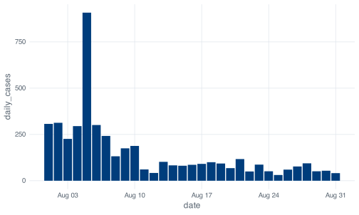
Note where the operators change. Every step up to ggplot() uses %>%, because each one takes a data frame and returns a data frame. Everything after uses +, because ggplot() returns a plot object and plot objects are built by addition. The change of operator marks the point where the data frame becomes a plot.
That figure also shows why 5 August carries a caveat throughout this book. The 908 cases that day were a reporting artifact from dormitory clearance testing rather than a day of unusually high transmission: 903 of the 908 were dormitory residents and 581 were linked to a single cluster at Acacia Lodge, and MOH attributed the batch to testing that picked up past infections. August’s median is 91 and the next highest August day is 313. None of that is visible in the bar chart; it has to come from the reporting around the data.
daily_casesWorked examples that already look right give little guidance on what to do when a plot comes out wrong, so this section starts from one that does and works through the available fixes.
The first thing to look at for any numeric variable is its distribution.
geom_histogram() will cut the range of daily_cases into 30 bins. Before you run the next chunk, commit to a number: how many of those 30 bars do you expect to be tall enough to see on the page? Write it down.
ggplot(covid, aes(x = daily_cases)) +
  geom_histogram()
#> `stat_bin()` using `bins = 30`. Pick better value `binwidth`.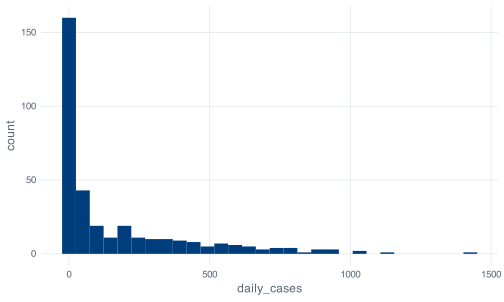
Only two bars have any visible height, and the rest are too short to read at a scale set by the tallest one. The message above the figure, `stat_bin()` using `bins = 30`. Pick better value `binwidth`., reports a decision ggplot2 made on your behalf. It uses 30 bins because a histogram needs some bin count, and it prints the message on every call so that the value it chose stays visible in your output.
Nothing went wrong in the code. The plot is an accurate picture of a variable that runs from 0 to 1,426 with a median of exactly 40. Bin one, covering roughly 0 to 25 cases, holds 160 of the 345 days. The top third of the range, everything above about 950, holds four days in total. Once one bar is 160 units tall, a bar of height 3 is two pixels.
ggplot(covid, aes(x = daily_cases)) +
  geom_histogram(bins = 60)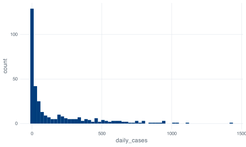
Doubling the bin count changes nothing that matters here, because resolution was not the problem. The shape is set by the range of the variable relative to where most of the mass sits, and the bin count changes neither.
ggplot(covid, aes(x = daily_cases)) +
  geom_histogram(binwidth = 25) +
  xlim(0, 400)
#> Warning: Removed 55 rows containing non-finite outside the scale range
#> (`stat_bin()`).
#> Warning: Removed 2 rows containing missing values or values outside the scale range
#> (`geom_bar()`).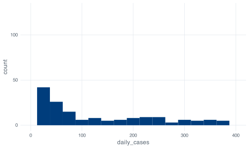
Now you can see the distribution, and R has warned you twice about what it cost. Fifty-five days, every day above 400 cases, were dropped before the bins were counted. The second warning is about the bar that straddled the 400 boundary and could not be drawn.
coord_cartesian() produces a similar-looking result by a different mechanism:
ggplot(covid, aes(x = daily_cases)) +
  geom_histogram(binwidth = 25) +
  coord_cartesian(xlim = c(0, 400))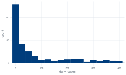
This time there are no warnings, because nothing was discarded. xlim() filters the data and then bins what survives; coord_cartesian() bins everything and then zooms the drawing. For a histogram the difference is real: with xlim() a bin near the boundary is computed from a truncated dataset, with coord_cartesian() it is computed from all 345 days and merely runs off the edge of the panel.
For both, the cost is that a reader of the finished figure does not see the warnings. A figure whose x axis stops at 400 implies that no day exceeded 400 cases. Fifty-five days did, one of them 1,426. A zoomed or truncated axis needs to be stated in the caption.
ggplot(covid, aes(x = daily_cases)) +
  geom_histogram(binwidth = 25) +
  scale_x_log10()
#> Warning in scale_x_log10(): log-10 transformation introduced infinite values.
#> Warning: Removed 13 rows containing non-finite outside the scale range
#> (`stat_bin()`).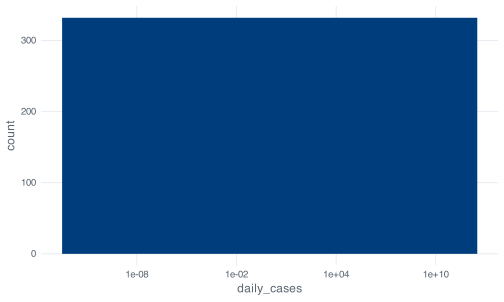
The cost is the 13 days with zero new cases, which are dropped, and both warnings tell you so. log10(0) is -Inf, and no axis has a position for negative infinity, so logging a count variable deletes every zero in it. Here that is 13 days out of 345, all of them in the first seven weeks of the record.
None of these fixes addresses the larger problem, which is that a histogram of daily_cases discards the date. The 345 values were not drawn from a single distribution: they come from a January with single-digit days, an April in which the dormitory outbreak took hold, and a November averaging under seven cases a day. Pooling them into one distribution describes a mixture of periods that differ from each other more than the values within any one of them differ.
Use a histogram for variables where the shape of the distribution is the question; the stringency index is one. For case counts, plot the time series.
hist() and its breaks argumentIf you have seen base R, you have seen hist(), and it takes an argument called breaks:
h <- hist(covid$daily_cases, breaks = 30, plot = FALSE)
length(h$counts)
#> [1] 29
The result is 29, not the requested 30. breaks is documented as a suggestion: base R passes your number to an algorithm that finds round-numbered cut points near it, and here that gives intervals of 50 from 0 to 1450. Ask for 30 and you get 29 whenever the rounded cut points imply a different count.
ggplot2’s bins argument is taken literally. Ask for 30 and you get 30, with bin edges at whatever values that implies: 49.17 wide, in this case, starting below zero. Neither behaviour is wrong. They optimise for different things, and confusing the two produces figures whose bins do not match the description in the text.
Start from the working plot and add the things a reader needs.
scale_x_date() controls where the tick marks go and how they are labelled. date_breaks takes a plain-English interval, and date_labels takes a strftime format string, the same one format() uses.
ggplot(covid, aes(x = date, y = daily_cases)) +
  geom_line() +
  scale_x_date(date_breaks = "1 month", date_labels = "%b")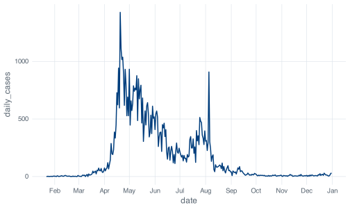
%b is the abbreviated month name.
Twelve labels is about the limit before they start colliding at this figure width. "2 months" with "%b %Y" is the version that survives being shrunk into a two-column manuscript. The interval string accepts "1 week", "3 months", "1 year" and so on, in the obvious way.
The format codes to remember are %b for Jan, %B for January, %d for the day number, %Y for a four-digit year and %y for two. ?strptime lists the rest.
geom_hline() draws a horizontal line at a value you choose. It is most useful for marking a threshold that already exists in the analysis, rather than one chosen to suit the figure.
The severity column built in the conditionals chapter calls a day High above 300 cases. Drawing that boundary makes the classification visible:
ggplot(covid, aes(x = date, y = daily_cases)) +
  geom_hline(
    yintercept = 300,
    linetype = "dashed",
    colour = nus_colours[["crimson"]]
  ) +
  geom_line() +
  scale_x_date(date_breaks = "2 months", date_labels = "%b %Y") +
  labs(x = NULL, y = "New cases per day")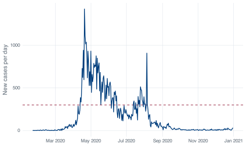
The geom_hline() comes before geom_line() in that call, and the order is deliberate. Layers are drawn in the order you add them, so a layer added later sits on top. Put the reference line last and it will cross over your data. There is no z-order setting; the order in the code is the order on the page.
geom_vline() is the vertical equivalent and takes xintercept. On a date axis it needs a real date object rather than a string that looks like one, and the failure is delayed until the plot is drawn:
ggplot(covid, aes(x = date, y = daily_cases)) +
  geom_line() +
  geom_vline(xintercept = "2020-04-07")
#> Error in `transformation$transform()` at ggplot2/R/scale-.R:1005:3:
#> ! `transform_date()` works with objects of class <Date> only
as.Date("2020-04-07") works. The underlying axis is a number of days since 1970-01-01, and a character string has no position on that line. The error surfaces at print time rather than when you write the layer, which is why a ggplot mistake sometimes appears several lines after you made it.
For a period rather than a moment, shade a rectangle:
ggplot(covid, aes(x = date, y = daily_cases)) +
  annotate("rect",
    xmin = as.Date("2020-04-07"), xmax = as.Date("2020-06-01"),
    ymin = -Inf, ymax = Inf,
    fill = nus_colours[["grey"]], alpha = 0.4
  ) +
  geom_line() +
  scale_x_date(date_breaks = "2 months", date_labels = "%b") +
  labs(x = NULL, y = "New cases per day")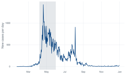
annotate() is for marks that are not in your data. It takes the geom name as a string and then fixed values rather than an aes() mapping, which is what you want for a one-off box. -Inf and Inf mean “the bottom and top of the panel, whatever they turn out to be”, so the shading keeps its full height if you later change the y limits.
geom_col() draws a bar whose height is the value in the data. geom_line() connects consecutive points. Choosing between them is a claim about what happens between your observations.
Over 345 days, geom_col() gives you this:
ggplot(covid, aes(x = date, y = daily_cases)) +
  geom_col() +
  scale_x_date(date_breaks = "2 months", date_labels = "%b")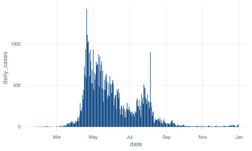
The result is defensible but hard to read: the bars are narrower than the gaps between them at this width, so the picket-fence effect carries visual weight that has nothing to do with the data. Bars are arguably the better match to what was measured, because each day’s count is a separate number and nothing was observed between Tuesday and Wednesday, whereas a line implies a continuous quantity sampled daily, which a notification count is not.
Lines carry a long daily series better; bars carry a short one, where each day is wide enough to be read on its own. Twenty-nine bars for August works. Three hundred and forty-five does not.
Aggregate first and bars come back into their own:
monthly <- covid %>%
  group_by(month) %>%
  summarise(cases = sum(daily_cases))

monthly
#> # A tibble: 12 × 2
#>    month      cases
#>    <date>     <dbl>
#>  1 2020-01-01    13
#>  2 2020-02-01    89
#>  3 2020-03-01   824
#>  4 2020-04-01 15243
#>  5 2020-05-01 18715
#>  6 2020-06-01  9023
#>  7 2020-07-01  8298
#>  8 2020-08-01  4607
#>  9 2020-09-01   953
#> 10 2020-10-01   250
#> 11 2020-11-01   203
#> 12 2020-12-01   381

ggplot(monthly, aes(x = month, y = cases)) +
  geom_col() +
  scale_x_date(date_breaks = "2 months", date_labels = "%b") +
  scale_y_continuous(labels = label_comma()) +
  labs(x = NULL, y = "Cases reported that month")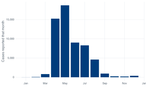
label_comma() comes from the scales package, loaded by _common.R. Without it that axis reads 0, 5000, 10000, 15000 and your reader has to count digits. Five-figure numbers on an axis should have separators.
Drawing those twelve monthly totals as a line would be a mistake. A line between May and June invites the eye to read a value for the middle of the month, and no such value exists: May’s number is a total for the whole month. Use bars for totals over a period and lines for quantities measured through time.
Bar charts need a y axis that starts at zero. What the reader compares is the length of the bar, so truncating the axis changes the ratios the figure appears to show in a way that truncating a line chart does not. coord_cartesian(ylim = c(4000, 20000)) on that plot would draw May at three times April’s height instead of 1.2 times.
Case counts spanning three orders of magnitude are what a log y axis is for. Try it:
ggplot(covid, aes(x = date, y = daily_cases)) +
  geom_line() +
  scale_y_log10()
#> Warning in scale_y_log10(): log-10 transformation introduced infinite values.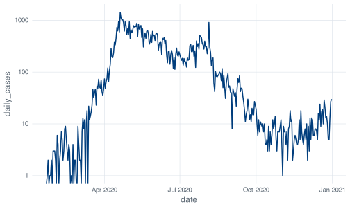
Warning in scale_y_log10(): log-10 transformation introduced infinite values. states the problem exactly. log10(0) is -Inf. Thirteen days in 2020 had zero new cases, all of them between 22 January and 12 March, and a log axis has no position for them, including at the bottom of the panel: a log axis has no lower end, because it extends towards negative infinity. The property that compresses large values is the same one that stretches small ones without limit.
No argument to scale_y_log10() fixes this, because the problem is arithmetic rather than a plotting decision. That leaves two options, and both are decisions about the analysis that belong in your methods section.
Plot cases plus one. Add 1 to every count so the zeros land at log10(1) = 0:
ggplot(covid, aes(x = date, y = daily_cases + 1)) +
  geom_line() +
  scale_y_log10() +
  scale_x_date(date_breaks = "2 months", date_labels = "%b") +
  labs(x = NULL, y = "New cases per day, plus one")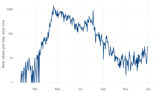
The distortion is largest where the data is smallest: a day with 1 case and a day with 2 cases are now 2 and 3, a ratio of 1.5 rather than 2. At 500 cases the shift is invisible. Whether that is acceptable depends on whether the low-count period matters to your argument; if the analysis concerns January, the adjustment is not neutral there. Either way the axis label and the caption have to state it, which is why the label above reads “New cases per day, plus one”.
Smooth first. A seven-day mean of this series never hits zero, because no run of seven consecutive days in 2020 was all zeros:
smoothed <- covid %>%
  mutate(
    cases_7day = as.numeric(stats::filter(daily_cases, rep(1/7, 7), sides = 1))
  )

smoothed %>%
  select(date, daily_cases, cases_7day) %>%
  slice(5:9)
#> # A tibble: 5 × 3
#>   date       daily_cases cases_7day
#>   <date>           <dbl>      <dbl>
#> 1 2020-01-26           1      NA
#> 2 2020-01-27           1      NA
#> 3 2020-01-28           2       1
#> 4 2020-01-29           0       1
#> 5 2020-01-30           3       1.29

ggplot(smoothed, aes(x = date, y = cases_7day)) +
  geom_line() +
  scale_y_log10() +
  scale_x_date(date_breaks = "2 months", date_labels = "%b") +
  labs(x = NULL, y = "New cases, seven-day mean")
#> Warning: Removed 6 rows containing missing values or values outside the scale range
#> (`geom_line()`).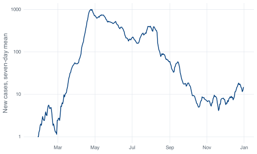
The warning about six removed rows is the first six days, which have fewer than seven days behind them. sides = 1 makes the window trailing, so each value averages that day and the six before it, which is what public health reporting means by a seven-day average. The default, sides = 2, centres the window and uses days that had not happened yet.
stats::filter() needs the stats:: prefix because dplyr’s filter() masks it. Drop the prefix and you get this:
filter(covid$daily_cases, rep(1/7, 7), sides = 1)
#> Error in `UseMethod()`:
#> ! no applicable method for 'filter' applied to an object of class "c('double', 'numeric')"
That is dplyr’s filter() reporting that it was given a numeric vector when it expected a data frame, in wording that gives no indication that a different filter() exists. The clash arises because both packages use the same name for different functions. The startup message printed when the tidyverse loads records which functions are masked.
Smoothing removes the spikes. The 5 August artifact, 908 cases in a month with a median of 91, becomes a modest bump once it is averaged with six ordinary days. If the spike is the subject of the analysis, smoothing hides it.
Both options change the quantity being plotted rather than only its appearance. Choose one, apply it before drawing, and describe it alongside the rest of your methods.
facet_wrap() splits one plot into small panels by the values of a variable. Every panel gets the same geom, the same mapping and, by default, the same axes, which is what makes the panels comparable.
covid %>%
  mutate(month_name = format(date, "%B")) %>%
  ggplot(aes(x = date, y = daily_cases)) +
  geom_line() +
  facet_wrap(~ month_name, scales = "free_x")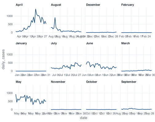
The panels come out in alphabetical order rather than calendar order: April, August, December, February, then January, July, June, March, then May, November, October, September.
format(date, "%B") returns a character vector, and R sorts character vectors alphabetically. ggplot2 has no way to know that these strings are months, so it does what it does with any character variable: converts to a factor, and factor() on a character vector orders the levels by sort().
No argument to facet_wrap() sets the panel order. The fix belongs in the data: a factor whose levels are in the order you want, built before the data reaches ggplot():
covid %>%
  mutate(
    month_name = factor(format(date, "%B"), levels = month.name)
  ) %>%
  ggplot(aes(x = date, y = daily_cases)) +
  geom_line() +
  facet_wrap(~ month_name, scales = "free_x")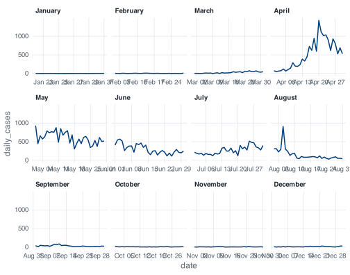
month.name is a built-in constant: a character vector of the twelve month names in calendar order, available in any R session without a package. Typing month.name at the console prints it.
Recognise order-of-levels problems as a category: they present as plotting bugs. Bars in the wrong order, legend entries in the wrong order and panels in the wrong order are all the same problem, and all are fixed in the data rather than in the plot. The severity column avoids it because covid_daily() builds it with factor(severity, levels = c("Low", "Medium", "High")) rather than letting R sort High, Low, Medium.
Two facet_wrap() arguments do most of the work. ncol (or nrow) sets the layout. scales decides whether panels share axes: "fixed" is the default and is what you want when the point is comparison; "free_x", used above, gives each month its own date range so the twelve panels do not each show ten days of line and eleven months of blank; "free_y" lets each panel find its own vertical scale, which makes small panels legible at the cost of comparability between panels. Free scales change what the figure can be used for, so choose them deliberately.
labs() sets every piece of text around the plot: the axis titles, the plot title and subtitle, the caption and the legend titles.
ggplot(covid, aes(x = date, y = daily_cases)) +
  geom_line() +
  scale_x_date(date_breaks = "2 months", date_labels = "%b") +
  labs(
    title = "Reported COVID-19 cases in Singapore, 2020",
    subtitle = "Daily counts, differenced from the cumulative confirmed series",
    x = NULL,
    y = "New cases per day",
    caption = "Source: COVID-19 Data Hub."
  )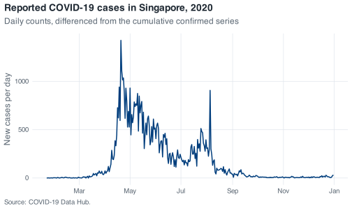
x = NULL removes the axis title rather than blanking it, which reclaims the space. Do that when the axis is self-evident, as a row of month names is. x = "" leaves an empty label and its margin behind, which is why plots sometimes have a mysterious gap at the bottom.
Default axis titles are the column names, so an unlabelled plot shows daily_cases on the y axis. labs() replaces it with wording a reader can interpret without access to the code.
The subtitle is the place for information the reader would otherwise have to ask for. This series is differenced from a cumulative column, and a reader needs to know that before interpreting the spikes.
facet_wrap() splits one plot by a variable. Every panel is the same plot with different rows.
Putting two different plots side by side is a different job, and facet_wrap() cannot do it. The base R answer was par(mfrow = c(2, 1)), which sets a global graphics parameter and stays set until you change it back, so an unrelated plot three commands later is still drawn into a two-panel layout. The tidyverse answer is patchwork, loaded by _common.R.
Build the plots as ordinary objects, then combine them with operators. / stacks, | puts side by side.
p_cases <- ggplot(covid, aes(x = date, y = daily_cases)) +
  geom_line() +
  scale_x_date(date_breaks = "2 months", date_labels = "%b") +
  labs(x = NULL, y = "New cases")

p_stringency <- ggplot(covid, aes(x = date, y = stringency_index)) +
  geom_line(colour = nus_colours[["crimson"]]) +
  scale_x_date(date_breaks = "2 months", date_labels = "%b") +
  labs(x = NULL, y = "Stringency index")

p_cases / p_stringency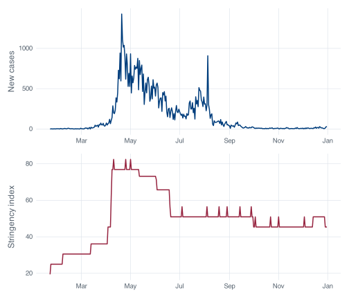
stringency_index is the Oxford Government Response Tracker’s summary of how restrictive a country’s policy was on a given day, on a 0 to 100 scale. In this file it runs from 19.44 to 82.41.
Stacked against the case curve, it shows something a single panel cannot. Stringency is a staircase, because policy changes on announced dates and holds until the next announcement, while the case series varies from day to day. The step on 7 April is the circuit breaker, and it is large: stringency goes from 45.37 to 62.04 in one day, retail mobility from -15 to -51, workplaces from -24 to -52. The index reaches its maximum of 82.41 for the first time on 10 April, three days later, and cases keep climbing for another ten days after that.
The small movements after July do not support interpretation. There are 23 changes in the index after 1 July, several of them one-day blips that cannot be distinguished from encoding artifacts. A single-day rise in a composite index is not evidence of a policy announcement.
Patchwork’s other operators are good to know. + packs plots into a grid and lets patchwork choose the shape, | forces a row, / forces a column, and they nest with brackets: (a | b) / c. plot_layout() controls proportions, and plot_annotation() adds text to the assembly rather than to any one panel:
(p_cases / p_stringency) +
  plot_layout(heights = c(2, 1)) +
  plot_annotation(
    title = "Cases and policy stringency, Singapore 2020",
    caption = "Sources: COVID-19 Data Hub; Oxford COVID-19 Government Response Tracker.",
    tag_levels = "A"
  )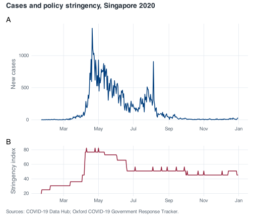
tag_levels = "A" labels the panels A and B, the labelling convention for multi-panel figures in published work.
Use facet_wrap() when it is one plot cut into pieces by a variable, and patchwork when it is several plots that belong on the same page. The usual symptom of choosing the wrong one is data reshaped into a long format so that two variables measured on different scales can be faceted against each other. If the panels need different y axes because they show different quantities, patchwork is the tool.
ggsave() writes the last plot, or a plot you name, to a file. Called with no dimensions it uses whatever your current graphics device happens to be:
out <- tempfile(fileext = ".png")
ggsave(out, plot = p_cases)
#> Saving 7 x 4.19 in image
Saving 7 x 4.2 in image reports the size R chose. It comes from the device open at the time, so the same script produces different files depending on how wide the RStudio plot pane happens to be. A figure whose size depends on the shape of a window is not reproducible, and the symptom is usually inconsistent font sizes between figures in the same document.
Give it dimensions:
ggsave(
  "figures/epi-curve.png",
  plot = p_cases,
  width = 7,
  height = 4.2,
  dpi = 300
)
width and height are in inches by default, and units = "cm" or units = "mm" changes that. Set them to the size at which the figure will be printed. A figure drawn at 12 inches and then shrunk into a single manuscript column has 6-point axis labels; the same figure drawn at 3.5 inches has readable text, because ggplot2 sizes the text relative to the canvas it is given. Size the figure for its final home rather than resizing it afterwards.
dpi sets the resolution of raster formats. 300 is the usual journal minimum for .png, 600 for figures with fine detail, and 96 is what you get by default, which is a screen resolution and will look soft in print.
The file extension chooses the format. Use .png for anything with many plotted elements and for slides. Use .pdf for line art going into a LaTeX manuscript, where it stays sharp at any zoom and dpi becomes irrelevant.
.svg needs the svglite package, which is not installed in this project:
ggsave(tempfile(fileext = ".svg"), plot = p_cases)
#> Saving 7 x 4.19 in image
#> Error in `dev()` at ggplot2/R/save.R:107:3:
#> ! The package "svglite" is required to save as SVG.
The error names the missing package, which is the pattern to expect from ggplot2 when a format needs a helper. install.packages("svglite") fixes it if you want SVG. When you install a package for a real project, record the addition afterwards with renv::snapshot(), so the project library stays pinned.
Saving a figure by right-clicking the plot pane and choosing Export produces a file at whatever size the pane happened to be, records nothing about how the figure was made, and has to be repeated by hand whenever the data changes. A call to ggsave() in the script regenerates the figure at a stated size every time the script runs. That is the property the report-rerun habit depends on: when the data changes and the script runs again, every figure saved by code is rewritten at its stated size by the same run that updates the tables and the numbers in the text, whereas a figure exported by hand has to be re-exported by hand and is easily forgotten.
Exercise 9.1 (Draw a publication-ready epidemic curve) Produce a single figure of daily reported cases across 2020 that a reader can interpret without additional explanation. It needs axis labels that are English rather than column names, month ticks that do not collide, a title, and a caption that says the counts were differenced from a cumulative series. Mark the circuit breaker period, 7 April to 1 June 2020, so the reader can see where it falls relative to the peak. Save it as a 300 dpi PNG at a size that would fit in a single column of a journal page, roughly 3.5 inches wide.
Then look at what your text does at that width and fix it.
Build the plot as an object first and print it, then pass that object to ggsave() with explicit width, height and dpi. Shading a date range is annotate("rect", ...) with ymin = -Inf and ymax = Inf.
Exercise 9.2 (Make the distribution legible, and say what it cost) The raw histogram of daily_cases is dominated by one bar. Produce a version a reader can actually learn something from, and write two or three sentences underneath it stating exactly which days are not represented and why.
Then produce a second version that splits the year into panels by month, using a factor so the panels come out in calendar order, and say which of the two you would put in a report and why.
There is no single correct fix here. binwidth, coord_cartesian(), xlim() and scale_x_log10() all change the picture and each one gives something up. Pick one, and let the warnings R prints tell you what to write in your two sentences.
Exercise 9.3 (Put policy next to cases) Build a two-panel figure with daily cases on top and stringency_index below, sharing a common date axis, labelled A and B, under one overall title.
Then answer in prose, from the figure: on what date does the stringency index first reach its 2020 maximum, and had daily cases peaked by then? Use the figure to form the answer and the data to check it.
Make two ordinary ggplot objects, then combine them with /. For the check, slice_max() on stringency_index will give you more than one row, so think about what arrange(date) does to that result.