1 Getting set up
This chapter installs two programs, in a particular order, and finishes with a check that they work together. The process takes about twenty minutes, most of which is downloading. If you already have both installed and working, skip to the check at the end of this chapter, run it, and move on.
1.1 R first, then RStudio
R is the language and the engine. It is what actually adds the numbers up. RStudio is a front end: an editor, a console, a plot viewer and a file browser stitched together into one window. RStudio does no statistics of its own. When it starts, it goes looking for an R installation on your machine and talks to it.
This is why R goes on first. If you launch RStudio with no R installed, it reports that it cannot find one and refuses to start. Install R, confirm it exists, then install RStudio.
R comes from CRAN, at https://cran.r-project.org. Pick your operating system from the links at the top.
On macOS you will be offered two installers and you have to choose. If your Mac has an Apple silicon chip (M1 and later), take the one whose filename contains arm64. If it is an older Intel Mac, take the x86_64 one. Apple menu, then “About This Mac”, tells you which you have. The wrong choice still runs, under emulation, but more slowly, and it causes trouble later when a package has to be compiled.
On Windows, follow “Download R for Windows”, then “base”, then the big download link. You may see a mention of Rtools on that page. You do not need it for this book. It is for compiling packages from source, which nothing here asks you to do.
On Linux, follow CRAN’s per-distribution instructions. Distribution repositories carry their own r-base package, and it is often several versions behind.
This book needs R 4.1 or newer. Anything from the last few years is fine.
RStudio comes from Posit, at https://posit.co/download/rstudio-desktop/. You want RStudio Desktop, the free open-source version. Posit also sells a paid tier and hosts a server edition, which run on the same editor and add features this book does not use.
Once both are installed, start your work from RStudio rather than from R. R ships with its own minimal window, RGui on Windows and R.app on macOS, which offers a console and little else; RStudio provides the editor, plot viewer and file browser that the rest of this book assumes.
1.2 The four panes
RStudio’s window is divided into four, and the first time you see it there is a lot going on. Here is what each one is for.
The Console, bottom left, is R itself. The > prompt is R waiting for you to say something. Type 1 + 1 there and press Enter and you get an answer. Everything that runs in this book runs through this pane, one way or another.
The Source pane, top left, is where your scripts live. It is empty when you first launch, because you have no scripts. Go to File, New File, R Script and it appears, pushing the console down into the lower half. This is where you will spend most of your time.
The Environment pane, top right, lists the objects R currently holds in memory: your data frames, your variables, anything you have created. It is the answer to “did that actually work?”. If you read a CSV and nothing shows up here, the read did not happen. The History tab next to it keeps a log of everything you have typed.
The bottom right pane is a stack of tabs: Files for browsing your folders, Plots for anything you draw, Packages for what is installed, Help for documentation, and Viewer for things like rendered Quarto pages. You will use Plots and Help constantly and largely ignore the rest.
If the layout does not suit you, Tools, Global Options, Pane Layout will rearrange it.
One piece of console behaviour comes up in the first hour, so recognise it now. If the prompt changes from > to +, R has judged your command incomplete and is waiting for the rest of it.
> mean(c(1, 2, 3)
+
+
That happens when you leave a bracket or a quote unclosed. Press Esc: the prompt returns to > and you can start the line again. Pressing Enter instead only adds further + lines, since R is still waiting for the missing closing character.
1.3 Three keyboard shortcuts
RStudio has hundreds of keyboard shortcuts and you can see the whole list with Alt+Shift+K on Windows or Option+Shift+K on a Mac. Learn three of them before you write anything.
Run the current line. Ctrl+Enter on Windows and Linux, Cmd+Enter on a Mac. Put your cursor anywhere on a line in your script, press it, and that line is sent to the console and executed. The cursor then drops to the next line, so you can run a script line by line by holding the shortcut down. If you have text selected, it runs the selection instead. This is the shortcut you will use most.
Run the current chunk. Ctrl+Shift+Enter, or Cmd+Shift+Enter. In a Quarto or R Markdown document, code lives in fenced chunks, and this runs the whole chunk your cursor is sitting in. It has no effect in a plain .R script, which has no chunks, and becomes useful once you start writing reports.
Insert the assignment arrow. Alt+-, or Option+-. It types <- with a space either side, which saves three keystrokes on an operator you will type constantly.
R uses <- rather than = for historical and practical reasons. Historically, R inherited the arrow from S, which was written on terminals whose keyboards, borrowed from APL, had a single ← key, so assignment cost one keystroke. The practical reason is that = already has a second job inside function calls, where it names arguments. Compare the two in one line:
The <- creates an object. The = sets an argument. Keeping them visually distinct lets you read a long function call and see which is which. This book uses <- throughout.
1.4 The console and the script
Everything you type in the console runs immediately and is then, for practical purposes, gone. The History tab does keep a record, but it is an undifferentiated stream of everything you tried, wrong attempts and typos included, in the order you happened to type them, which leaves you to reconstruct the analysis from it afterwards.
A script is a file. It runs top to bottom in a fixed order. You can open it in six months, send it to a co-author, put it in a repository, and re-run it to get the same numbers.
Use the console for inspecting the data to see what is in it: nrow(covid), names(covid), checking whether a column is a character or a number. These are questions whose answers you will not need again. Anything you would have to redo, or would need to defend, goes in the script; a line you had to stop and think about is exactly the kind of line to keep in a file.
The awkward case is the analysis that lives entirely in the console. It works until R restarts, at which point the objects are gone and there is no record of how they were made.
1.5 Packages, install.packages() and library()
Base R can do a great deal, and it is deliberately conservative about what ships in the box. Most of what you will want lives in a package, and packages come from CRAN, the Comprehensive R Archive Network. CRAN is a network of mirror servers holding many thousands of packages, each of which has passed an automated check on several operating systems before being accepted. That check is the reason install.packages() from a fresh R install usually works without further configuration.
There are two functions involved, and they do different things.
install.packages("tidyverse") downloads the package from CRAN and writes it to your hard disk. You do this once per machine. It takes a while, especially for the tidyverse, because the tidyverse is a meta-package: installing it installs about thirty others.
install.packages("tidyverse")library(tidyverse) loads an already-installed package into your current R session, so its functions become available by name. You do this every session, at the top of every script. Restart R and it is undone.
The usual analogy is a bookshelf: install.packages() buys the book and puts it on the shelf, while library() takes it down and opens it, which is why the first runs once per machine and the second runs at the top of every session.
The quoting is inconsistent between the two, which is a common source of confusion. install.packages() requires quotes, because it takes the package name as a character string. library() does not, because it evaluates its argument non-standardly and accepts a bare name. Both accept quotes, so quoting in both places is a safe habit if you would rather not remember which is which.
When you run library(tidyverse) in a fresh session, this appears:
── Attaching core tidyverse packages ──────────────────────── tidyverse 2.0.0 ──
✔ dplyr     1.2.1     ✔ readr     2.2.0
✔ forcats   1.0.1     ✔ stringr   1.6.0
✔ ggplot2   4.0.3     ✔ tibble    3.3.1
✔ lubridate 1.9.5     ✔ tidyr     1.3.2
✔ purrr     1.2.2
── Conflicts ────────────────────────────────────────── tidyverse_conflicts() ──
✖ dplyr::filter() masks stats::filter()
✖ dplyr::lag()    masks stats::lag()
ℹ Use the conflicted package (<http://conflicted.r-lib.org/>) to force all conflicts to become errors
Your version numbers will differ. The red crosses are not errors. They report that dplyr has a function called filter() and so does base R’s stats package, and that since dplyr was loaded second, typing filter() now calls dplyr’s. That is the version this book uses, and R reports the substitution rather than making it silently. If you need the other one, stats::filter() names it explicitly. The :: means “this function, from that package”.
Read the block when it appears. When a function behaves unexpectedly, masking by a later-loaded package is a common explanation, and the conflicts list is where it was announced.
1.6 Getting the data
The book runs on one file, sg_covid_data.csv. It was assembled from three sources: the COVID-19 Data Hub R package (Guidotti & Ardia, 2020), the Oxford COVID-19 Government Response Tracker (Hale et al., 2021) and Google’s COVID-19 Community Mobility Reports; Appendix B gives the full citations. There are two ways to get it.
The thorough way is to take the whole book. Go to https://github.com/CERM-NUS/r-intro, click the green Code button, choose Download ZIP, and unzip it somewhere you will find again, such as your Documents folder rather than Downloads. You now have the data, the source of every chapter, and a .Rproj file. Double-click r-intro.Rproj and RStudio opens with everything pointed at the right place.
The quick way is to take just the CSV, from https://raw.githubusercontent.com/CERM-NUS/r-intro/main/data/sg_covid_data.csv. The “Download the data” link in this book’s sidebar points to the same address. Right-click, Save Link As. Then make yourself a folder for this course with a data subfolder inside it, and put the CSV in there:
sph5421/
├── data/
│   └── sg_covid_data.csv
└── analysis.R
Two warnings about that download. Some browsers append .txt to files they treat as plain text, so check that what landed on disk is called sg_covid_data.csv and not sg_covid_data.csv.txt. Second, avoid opening it in Excel to inspect it. Excel offers to save the file back on closing, and saving can rewrite the date column into whatever format your regional settings prefer. To look inside the file, read it into R instead: read_csv() reads the file and does not write to it. The raw file is never edited; every repair to the data happens later, in code. That is what the check below does.
1.7 Make the folder a project
With the folder made, turn it into an RStudio project. Go to File, New Project, Existing Directory, browse to the course folder, and click Create Project. RStudio closes and reopens inside the project, and an .Rproj file appears in the folder.
The .Rproj file does three things for you. R now starts with that folder as its working directory, so data/sg_covid_data.csv resolves without a path being typed. The project gets its own R session and its own command history, separate from anything else you have open. And it marks the folder: from now on you open the work by double-clicking the .Rproj file, and everything starts pointed at the right place. If you took the ZIP download in the previous section, you already have a project file, r-intro.Rproj, and can skip these steps.
1.8 Does it work?
Open a new script with File, New File, R Script; the green-plus button at the top left of the toolbar does the same thing, as does Ctrl+Shift+N, or Cmd+Shift+N on a Mac. Save it straight away with File, Save, naming it analysis.R — with a project open, the save dialog already starts in the project folder, so the folder ends up matching the tree shown in “Getting the data”. Then type the following in, and run it a line at a time with Ctrl+Enter, or Cmd+Enter on a Mac.
library(tidyverse)

covid <- read_csv("data/sg_covid_data.csv")
#> Rows: 345 Columns: 13
#> ── Column specification ────────────────────────────────────────────────────────
#> Delimiter: ","
#> chr   (1): administrative_area_level_1
#> dbl  (11): confirmed, deaths, stringency_index, government_response_index, c...
#> date  (1): date
#>
#> ℹ Use `spec()` to retrieve the full column specification for this data.
#> ℹ Specify the column types or set `show_col_types = FALSE` to quiet this message.

nrow(covid)
#> [1] 345
You should get 345, and above it a column specification listing 13 columns: one character, eleven numbers and one date. That block is readr reporting what type it assigned to each column. The types are inferred from the first thousand rows, so the block is where a wrong inference can be caught, rather than four steps into an analysis when a column that should be a date turns out to be text.
You will also see the tidyverse startup message from the previous section. It does not appear on this page because the machine that built the book had already loaded the tidyverse before this chapter started, and a package announces itself only the first time a session attaches it.
Now check that graphics work:
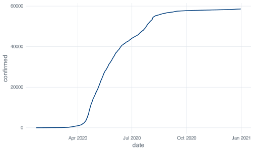
A line should appear in the Plots pane, climbing from zero in January to just under sixty thousand by December. Yours will have ggplot2’s default grey background, whereas the figures here do not, because the book applies its own theme to every figure. The data and the geometry are the same.
If the plot does not appear and the Plots pane looks squashed, drag the divider between the panes to make it taller. RStudio cannot draw into a pane a few pixels high.
1.8.1 When it does not work
Three failures account for nearly all of them.
Error in library(tidyverse) : there is no package called ‘tidyverse’The install did not finish, or finished with an error you scrolled past. Run install.packages("tidyverse") again and watch the output this time. On Windows, if it complains that the package is in use, restart R first.
Error:
! 'data/sg_covid_data.csv' does not exist in current working directory:
  '/Users/you/Desktop'.
R is looking in the wrong place. The message reports the directory it searched, so either the file is not where you think it is, or R’s working directory is not where you think it is. getwd() reports the current working directory:
getwd()
#> [1] "/Users/smishra/Documents/GitHub/r-intro"
Yours will print something else. The fix is a project file rather than a call to setwd(), whose path is specific to one machine and to the current arrangement of its folders. If you skipped “Make the folder a project” above, go back to it now: with a project open, R’s working directory is the project folder, and data/sg_covid_data.csv resolves without a path.
Error: unexpected input in "covid <- read_csv(“"Something in the line is not valid R. That particular one is a smart quote, the curly “ that Word and Slack substitute for the straight ". R does not recognise it as a quote character at all. If instead you left out a comma you get its sibling:
Error: unexpected symbol in "covid <- read_csv("data/sg_covid_data.csv" nrow"Both messages quote your line back and stop at the point where the parser failed, so the fault is usually immediately before that point.
If none of those match what you are seeing, copy the error text exactly, with your own file paths and object names removed, and search for it.